GETTING STARTED WITH SUPERCOMPUTING

Example #1: Missile Trajectory Simulation

1.0 Introduction

This example investigates a standard physics problem of missile trajectory, the typical scenario of a projectile launched toward a target which is a known distance away. The problem is to find which combinations of launch angle and corresponding velocity would be needed in order for the projectile to land arbitrarily close to that target. However, instead of solving the problem analytically [11], the following presentation uses a computational science approach.

2.0 Equations of the Model

As shown in figure 1, the height y of the projectile at time t is defined as:

y = v_y * t - 0.5 * a * t²

where v_y is the component of velocity in the vertical direction and a is the acceleration toward earth by the force of gravity.

Figure 1: Basic Model Parameters

The horizontal distance x travelled during time t is defined by the simple equation:

x = v_x * t

where v_x is the component of velocity in the horizontal direction.

Given the initial velocity v and launch angle theta, the components of velocity can be obtained using simple trigonometry:

v_x = v * cos(theta)

v_y = v * sin(theta)

3.0 Model Prototype
3.1 Creating the Initial Prototype

The first step in creating a computational model is to develop a simple prototype and then validate it against known behavior. For this example, a possible first stage might be to display a simple graphic showing the position of a projectile over time given an initial velocity and launch angle. The number of points plotted on the screen depends upon the time step, or the length of time between successive values of t. The following pseudocode describes the basic algorithm.

Enter Values:

v (velocity),
theta (launch angle),
dist (target distance),
range (error margin or acceptable radius for "hit" )

Initialize Variables:

t=0 (time),
tstep = 0.1 (time step between calculations)
a=32 (Gravitational constant in ft per sec2)

Find velocity components:

v_x=v*cos(theta)
v_y=v*sin(theta)

Loop through all combinations:

Repeat

t = t + tstep (Increment time step)
y = v_y * t - 0.5 * a * t * t (Calculate height)
x = v_x * t (Calculate horizontal distance )
plot(x,y) (Plot position of projectile )

Until y <= 0 (Until missile has hit the ground)

Test for accuracy:

If Abs(x-dist) < range

then result = Hit
else result = Miss

Figure 2: Trajectories at 60 Degree Angle
140 ft/sec and 150 ft/sec

Projectile Hits the Target at 150 ft/sec at an angle of 60 degrees

Figure 2 shows the plot of a projectile shot at two different velocities but at the same angle of 60 degrees. The distance to the target for the simulation is 600 feet, the error margin was 20 feet, and the time step was 0.2 seconds. Notice that a projectile fired at 150 ft/sec would hit the target whereas an attempt at 140 ft/sec would fall short of the mark.

3.2 Validation of the Prototype

Validation of a computer simulation model is one of the most important steps of any investigation. No matter how intricate a model might be, if that model does not adequately define the situation, there is no sense in drawing any conclusions from the simulation. In all computer models, there are certain simplifying assumptions that must be made since it is not possible to accurately simulate every single detail. Therefore, it is important that these simplifications do not interfere with the integrity of the model.

In this example, one possible behavior to validate is that the flight path of the projectile follows an expected parabolic curve. This can be done graphically. Another detail to establish is an appropriate time step between consecutive values of t in order to have predictable results when the projectile finally hits the ground. The time step could be made extremely small to increase accuracy, but that would make the execution time of the simulation much greater. Supercomputers are able to calculate at very rapid speeds, but there is no sense in wasting computer cycles unnecessarily.

To be sure that the model works correctly, it should be tested with several combinations of parameters where the behavior can be carefully analyzed and compared with known results. Good values to check are examples from mid-range as well as the extremes. Deviations from known behavior must be studied carefully and any problems corrected if the results are to be meaningful.

4.0 Expanding to a Supercomputer Application

Modern supercomputers are able to compute at hundreds of millions to even billions of calculations per second. Yet, unless algorithms are designed properly, much of that potential will never be accessed. The key to unleashing the computational power of most supercomputers is to find a way to do many similar calculations in parallel. Some supercomputers use a technique called vectorization which handles arithmetic with large arrays using a method similar to an assembly line. In other supercomputers, the same primary calculation is done by many separate processors simultaneously, but with different initial values.

The basic prototype simulation runs easily on a microcomputer and certainly does not require a supercomputer. However, to make this a supercomputer application, the problem can be expanded to compare a full an entire range of velocities between 0 and 1000 feet per second with all possible launch angles between 0 and 90 degrees. That is a lot of calculations, but a supercomputer should be able do much of the work in parallel in order to produce results more rapidly. The desired outcome showing a complete picture of acceptable combinations is very computationally intensive, but just right for a supercomputer.

5.0 Displaying Results

To analyze the results, it would be possible to print a list of ordered pairs that are solutions, but a better approach might be to select a visualization technique using graphics. The method chosen for this example uses each pixel position on the screen to represent a different combination of distance and launch angle. Horizontal pixel coordinates stand for different velocities and vertical coordinates represent variations in launch angle. There are many combinations to try, and thus, very many simulations to run. In standard VGA graphics, there are 640 pixels horizontally by 480 pixels vertically, or 307,200 combinations. A supercomputer may be able to do many of these calculations simultaneously, although a standard PC would have to try each combination separately.

For each of the defined positions, the prototype model described earlier must go through its full simulation and then decide whether the combination of parameters produced a hit or miss. The screen position is then colored differently depending upon the result: a darker shade for a hit, or two alternating lighter shades for a miss.

The graphic image in figure 3 shows the results for the expanded model. The horizontal axis represents velocity, the vertical axis represents launch angle, and the solution set is clearly visible by the dark curved line. However, the simulation took several hours to complete on a PC running Turbo Pascal, and any enhancements would make execution time even longer. Therefore, it is a perfect candidate for a supercomputer application.

Figure 3: Computational Science Solution
Angle vs. Velocity

An interesting byproduct of the graphics visualization process in this example is the unusual pattern in the background. The design happens because the simulation plotted alternating colors for various distances which missed the target. The pattern is a function of not only how often the color changes (every foot versus every ten feet), but also the value used for the time step in the simulation.

6.0 Comparison to the Analytical Solution

There is also a purely mathematical solution to this investigation which is not too difficult to derive. Using the basic equations of the model combined with the fact that when the projectile strikes the target, the vertical height is zero yet the horizontal length equals the distance from source to target, it is possible to solve a system of equations which can be resolved into one form defining velocity in terms of launch angle, given various constants for target distance and gravitation. That relationship produces a graph that shows the same solution set described by the computational approach. It is defined by the following equation:

v = SQRT(( a * dist)/(2 * SIN(theta) * COS(theta)))

So why use a computational model when mathematical solution is obviously more exact? For one reason, if there is desire to expand the model to include other factors such as wind resistance, spins, bounces, and interference with various obstacles, then an analytical approach becomes increasingly more difficult. However, modifications to the computational model are comparatively easy since only additions to the basic simulation need to be defined.

There are times when the computational model may be the only alternative. In fact, some situations which seem relatively simple cannot be solved analytically at all. During the first SuperQuest contest, former student Eric Scheirer developed a new technique [20] to analyze one such unsolvable problem, the classic "three body problem". The difficulty in finding an analytical solution for three planets having mutual gravitational attraction is related to their interdependencies of that gravitational pull. Using a supercomputer simulation and a graphics display technique similar to the trajectory model, Eric was able to gain a partial understanding of the dynamics of that system.

Computational models are not fool proof either, for there are often difficulties with chaotic behavior and sensitivity to initial conditions. However, a carefully designed computational approach can often provide some insight into many "unsolvable" problems in mathematics and science.

7.0 Understanding the Trajectory Model

There are several things that the missile trajectory investigation can show. The visualization technique not only defines acceptable values for velocity and launch angle by means of a graph, but also shows that for a broad range of angles on either side of 45 degrees, the velocity required for a hit is not nearly as sensitive as it is at the extremes. When the angle approaches either zero degrees or 90 degrees, a slight change in angle requires a significant change in velocity in order to make a hit. This relationship, although intuitively obvious, is very clearly shown by the compu ter graphics.

Computational science models can provide alternative methods for investigating problems of all kinds. With the aid of graphics visualization, scientists can often gain additional insight into many research investigations. Sometimes an unrelated aspect of the display, such as the patterned background in the trajectory example, might be the inspiration for yet another project.

8.0 Extensions to the Basic Model

After students are introduced to the simple trajectory model, they are expected to make the model more complex by adding obstacles that could interfere with the path of the projectile. Students could add walls, objects that had gravitational fields, or any creative physics principle they wished.

Below is an example project by student Tom Dixon demonstrating the effects of a gravitational attractor deflecting the path of a projectile.

Projectile Deflected by a Gravitational Attractor
Normal Plot of Solution Set	Effects of Gravitational Attractor

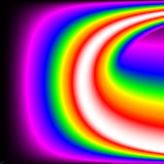
The following is an example by student David Rosenthal that shows the effect of a repelling influence. The white region indicates the combinations that were closest to the target, with the color gradations showing relative distances from the target. Notice the deforming of the solution set due to a gravitation-like influence that repulsed the object rather than attracting it.

Normal Simulation

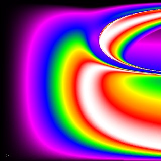
Repelling Influence